Dr. Martin Morgan is Professor of Oncology at Roswell Park Comprehensive Cancer Center, and led the Bioconductor project for 12 years. In this guest blog post, Dr. Morgan gives us an overview of the R / Bioconductor AnVIL package and shows how his group’s work empowers researchers to work more easily on the cloud.
The R / Bioconductor project started in 2001 as an effort to enable statistical analysis and comprehension of high-throughput genomic data. The project has grown from a small group of academic researchers to a global developer and user community engaging in challenges at the forefront of single cell expression, epigenomics, microbiome analysis, and many additional areas. The project consists of 2042 R software packages, in addition to ‘annotation’ and ‘experiment’ data resources to facilitate communication of statistical insights to the broader community of bioinformatics researchers. The project is very widely used (downloaded to more than 800,000 unique IP addresses in 2020) and highly respected (49,000 PubMedCentral full text citations), supporting academic, government, and industry researchers.
Many Bioconductor packages and community conferences have their own sticker, sharing a common hexagonal design. See the full list of available sticker images at https://github.com/Bioconductor/BiocStickers.
The Bioconductor community pioneered many best practices in research software development and dissemination, including fully open development of version controlled software, nightly builds and formal testing across multiple computer architectures, comprehensive help pages and ‘literate programming’ vignettes for all packages, and a standardized release cycle and distribution mechanism. Our community interacts through a support site, slack and email, and annual conferences in North America, Europe, and Asia. My group has been responsible for core development activities, with additional contributors at other institutions in the US and across the globe.
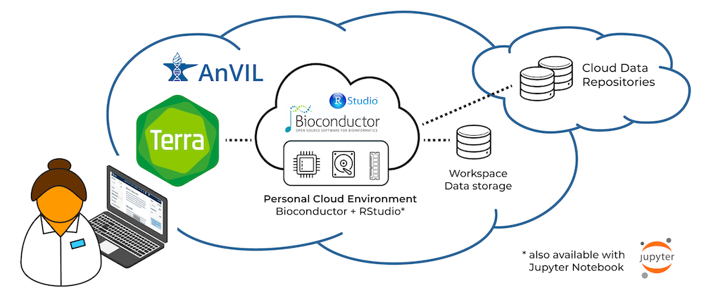
We participate in the AnVIL project as one way to engage in robust, scalable, and secure use of our software in a cloud-based environment. For several years, we’ve been working with our AnVIL partners to make R and Bioconductor available in Terra’s interactive cloud environment.
A researcher can now create an environment that includes core R / Bioconductor packages, as well as system dependencies to install virtually all Bioconductor packages, in just a few clicks. Researchers can use R / Bioconductor in either Jupyter Notebooks or RStudio, in a secure cloud environment. These environments are highly customizable, so researchers can adjust computational resources to fit their project requirements, and can easily and quickly install additional R / Bioconductor packages.
To learn more about Terra’s cloud environments framework, see Understanding and adjusting your Cloud Environment in the Terra documentation.
We developed the R / Bioconductor AnVIL package with three objectives in mind. First, the cloud offers unique features, e.g., a standardized computational environment, that we would like to exploit for the benefit of our users. Second, the cloud has features that are different from those in desktop or traditional high-performance computing environments, such as storage ‘buckets’ distinct from local runtime ‘disks’, and we would like to make these features accessible to our users through familiar R paradigms. Third, the Terra / AnVIL environment introduces approaches to data organization and secure access that benefit from an R interface to allow straight-forward use. We illustrate a few typical use cases in the following; we emphasize an RStudio environment, but most features are equally accessible in Jupyter notebooks running R kernels.
Using R / Bioconductor in the AnVIL cloud
Familiar ways of interacting with R on the desktop are replaced in Terra / AnVIL by account creation, selection of a workspace, and configuring and launching a cloud computing environment. There are excellent resources available for these steps; see for example RStudio in Terra blog post, and the Bioconductor tutorial workspace. In just a few minutes, the researcher is using a familiar RStudio environment with access to 1 to 96 CPUs, 3.75 to 624 GB memory, and 50 GB to a very large amount of disk space.
The following usage examples assume that we have cloned the public Human Cell Atlas (HCA) Optimus workspace, and started an RStudio cloud environment.
Terra / AnVIL RStudio is configured using a docker image that standardizes the compute environment. The image contains the current release version of R; a number of essential R packages are pre-installed.
library(tidyverse)
library(Seurat)
The universe of R and Bioconductor packages is large, so not all packages are installed ‘out of the box’. Instead, the computational environment contains system software that allows most packages to be installed quickly and easily. Start by installing the ‘devel’ version of the AnVIL package from its GitHub repository (the R / Bioconductor AnVIL package continues to change in response to the most recent features in Terra / AnVIL) using standard Bioconductor procedures:
BiocManager::install("Bioconductor/AnVIL")Notice that several packages are installed with AnVIL. In the RStudio image, these packages are installed as ‘binaries’ — no compilation is required! This is an important consequence of the standardized compute environment brought to us by the cloud. The AnVIL package allows us to quickly install Bioconductor (and CRAN R) packages in a fast and robust manner.
AnVIL::install(c("SingleCellExperiment", "LoomExperiment"))In RStudio, this installs about 20 Bioconductor and CRAN packages in just about as many seconds. A traditional installation would take several minutes, and possibly require installation of system dependencies — taking many more minutes, and requiring ‘super user’ access and advanced operating system knowledge. As an added benefit, the packages themselves are downloaded quickly, because the binary package repository is also located in the Google cloud.
The AnVIL::install() command illustrates how standardized computational environments configured by experts can be exploited to allow features such as robust, fast software installation by non-expert users.
Mastering cloud data storage concepts
Cloud computing adds new concepts to familiar computing paradigms. One example is the storage ‘bucket’. Buckets can be used for long-term storage of research data, including data files generated by labs or consortia that the researcher is involved with. Buckets exist independently of the cloud computing environment, with access either open to the public or restricted to specific groups or individuals. For instance, 1000 genomes data at gs://genomics-public-data/1000-genomes/ is in a publicly accessible bucket; files stored in the bucket can be copied to the local disk for processing, e.g., input into R using standard tools:
## retrieve the 1000 genomes 'sample_info.csv' file
src <- "gs://genomics-public-data/1000-genomes/"
sample_info <- paste0(src, "other/sample_info/sample_info.csv")
AnVIL::gsutil_cp(sample_info, "sample_info.csv")
csv <- readr::read_csv("sample_info.csv", guess_max = 5000)
AnVIL::gsutil_cp() performs the copy operation by invoking a function from the ‘gsutil’ software provided by the Google Compute Cloud and installed on the RStudio docker image. Similar functionality exists for listing bucket content, ‘piping’ content directly into R without creating a local copy, and synchronizing (e.g., backup or restore) the local file system with buckets. Data movement from buckets to the local disk are usually very fast, because transfer is within the Google cloud.
Terra / AnVIL allows groups of users, e.g., members of the same lab, to easily and securely share data with one another. Each Terra / AnVIL workspace has a bucket associated with it; access to the bucket is restricted to users with access to the workspace. This could be a single individual, a lab group, or a larger collection of Terra / AnVIL users. The path to the workspace bucket is available within AnVIL:
AnVIL::avbucket()The content of the bucket, or arbitrary paths in the bucket, are easily listed and copied to the local disk using commands like gsutil_ls(), gsutil_cp(), and gsutil_localize(), mentioned above.
Terra / AnVIL also provides facilities for gaining access to consortium or otherwise restricted data, e.g., through dbGaP authentication. Functions such as AnVIL::gsutil_cp() use Terra / AnVIL credentials, so the researcher can access any bucket the Terra / AnVIL account has access to.
Consortium-based resources often restrict access to authorized users. These resources are increasingly accessible through ‘DRS’ (Data Repository Service) addresses. The blog post Embracing DRS URIs and the benefits of data interoperability standards explains DRS in greater detail. The following command obtains a description of a DRS resource, and then retrieves it for local use.
## A GTEx resource, requiring authentication
src <- "drs://dg.ANV0/00008531-03d7-418c-b3d3-b7b22b5381a0"
AnVIL::drs_stat(src) |> glimpse()
AnVIL::drs_cp(src, "my_drs_resource")
This particular example requires an active AnVIL account link as explained in this documentation article.
Interacting with Terra / AnVIL data models
Terra / AnVIL workspaces introduce novel features to help structure and disseminate data, especially for use in large-scale workflows. One of these is a system of data tables, or “data model”, that provides a way of organizing metadata about the data in a workspace, including the bucket location of files associated with each participant, sample, etc. For instance, the HCA Optimus workspace contains, under the ‘Data’ tab, tables describing ‘participant’, ‘sample’, and ‘sample_set’.
The data model system is particularly relevant to running large-scale workflows, which is beyond the scope of this blog post (see Workflows QuickStart Tutorials). However, it’s interesting to note that workflows can be launched on multiple entries in a table (for example, to launch the same workflow on multiple samples) and that the outputs of the workflows are written to the workspace bucket, and added to the data tables.
It can be very convenient to view, manipulate, and update this metadata using R. The following commands query for existing tables, then downloads the ‘sample’ table as a ‘tibble’ (data.frame).
AnVIL::avtables()
sample <- AnVIL::avtable("sample")
The metadata can be manipulated (e.g., combined with results of a workflow or with the researcher’s own data) using standard R commands. Use avtable_import(), avtable_import_set(), and avtable_delete_values() to add or update tables, or to delete values from an existing table.
It’s also possible to interact with the metadata in a different workspace. For example, set the default workspace to point to the original HCA analysis, which includes a number of workflow jobs.
AnVIL::avworkspace("featured-workspaces-hca/HCA_Optimus_Pipeline")This shows an interesting and flexible feature: data from one workspace is easily available in another, making it very easy to integrate data and analyses across workspaces.
The following commands provide a tibble describing all workflows that have been run, and the files associated with the most recent job
## a tibble describing 13 workflow jobs in the HCA workspace
AnVIL::avworkflow_jobs()
## a tibble describing the 174 log and output files produced by the most recent job
AnVIL::avworkflow_files()
The files can be manipulated using standard R commands, and gsutil_cp() or localize() used to copy relevant files to the local disk for processing, e.g. retrieving the ‘loom’ output file.
## describe files associated with the most recent job. '|>' is the
## pipe operator introduced in R-4.0. We use 'dplyr' commands to work
## with the tibble (data.frame) of files, but could as easily use
## base R commands
files <- AnVIL::avworkflow_files()
path <-
    files |>
    filter(endsWith(file, "loom")) |>
    pull(path)

## copy the loom file from the bucket to the local disk
local_loom <- basename(path)
AnVIL::gsutil_cp(path, local_loom)
A good next step might input the data into R for further analysis and visualization
library("LoomExperiment")    # Installed previously with AnVIL::install()
loom <- LoomExperiment::import(local_loom)
Summary
This blog illustrates how the R / Bioconductor AnVIL package empowers researchers by exploiting unique opportunities provided by standardized cloud-based deployments (e.g., fast, robust binary package installation); makes cloud-based concepts like storage buckets accessible from R; and facilitates interaction with unique Terra / AnVIL features like data tables and workflow outputs. The AnVIL package is mature and well-documented, so be sure to review the introductory vignette and reference manual. Ask questions on the Bioconductor support site or #anvil slack channel. The most recent ‘devel’ version of the package is available on GitHub; we look forward to your bug reports and feature requests!
Acknowledgements
The AnVIL package and additional infrastructure represents work of many individuals, including (in alphabetical order) Vincent Carey, Sweta Gopalakrishnan, Kayla Interdonato, Valerie Obenchain, Marcel Ramos, Sehyun Oh, Lori Shepherd, BJ Stubbs, Nitesh Turaga, and Levi Waldron.
Resources
Package doc page — https://bioconductor.org/packages/AnVIL.
Previous blog with video — https://terra.bio/try-rstudio-in-terra/
Bioconductor project — https://www.bioconductor.org/about/