In this guest blog post, Tiffany Miller describes an analysis project she undertook in Terra in collaboration with her colleague Mark Walker, in which they applied a metagenomic approach to identify viral insertion sites in human genome sequencing data (shared in this workspace). Tiffany is the manager of the Frontline Support team, and Mark is a data scientist in the GATK team; both teams are part of the Data Sciences Platform at the Broad Institute.
If you’ve ever emailed the Terra helpdesk or asked a question in either the Terra or the GATK forum, you’ve encountered my team, Frontline Support. Our core responsibility is to help researchers who are using GATK and/or Terra solve any problems they encounter so they can get their work done. As the team manager, I don’t get that much hands-on-keyboard time with the tools, so I like to take on side projects where I do some kind of analysis myself. It helps me stay up to date on the latest Terra functionality, since the platform evolves on an ongoing basis, and gives me insight into the user experience, which informs our support policies.
Most recently, I worked on a project with my colleague Mark Walker from the GATK development team. One of Mark’s signature contributions to GATK is a method called PathSeq, which enables you to extract and identify genomic sequences from microbial pathogens present in eukaryotic genomes, as described in this paper. I was lucky to get to know Mark two years ago when we taught a GATK workshop together; I had been looking for an opportunity to do a scientific project in Terra, so Mark suggested trying to apply the PathSeq method to a use case that he had not explored in his original work: detecting insertion sites of a viral genome such as HPV in a human genome. Since I’m not a scientist by training, Mark mentored me and guided the project.
I learned a lot about writing workflows and building a reproducible workspace in Terra by doing this project. So I thought I would share how Mark and I approached the work and implemented the analysis, breaking down the problem from beginning to end, in the hope that it might help some of you who are new to the platform and face similar challenges.
Scoping the project
We started out by outlining the steps that would take us to our end goal:
- Create synthetic data with a known insertion site
- Run Pathseq on the synthetic data using a virus-only microbial reference
- Evaluate whether Pathseq had identified the synthetic insertion correctly by examining results visually in IGV
- If yes, find a way to identify the insertion site in the human data programmatically
- Develop a way to visualize the insertion site information conveniently
This would be our roadmap that we’d come back to frequently in our notes document. Every time we met we took notes and expanded on the details of the next steps to trigger our memory. This was helpful since most of the work was done asynchronously and neither of us had a ton of time to work on it. We decided on a bi-weekly schedule to meet for troubleshooting and to review progress. This was a good way to hold ourselves accountable to the project.
Creating the synthetic test data
We needed a test dataset with a known insertion, but couldn’t find anything suitable in the public domain, and we didn’t want to have to deal with restricted access data. So we decided to just create some synthetic human genome data to which we would add the viral genome and thus create an appropriate test case. As a direct benefit of that approach, our test case would be publicly shareable and reusable by anyone else.
Specifically, we decided to use the virus sequence HPV16 (retrieved from Refseq) and insert it in the p53 gene on chr17 of the hg19 reference genome. We also decided to use 30x coverage, which is standard in the field of human genomics, and to generate genome data for that chromosome only, to keep the sample file small for convenience.
Harnessing and extending existing synthetic data generation tools
I knew that others in our team had written WDL workflows to generate synthetic data for a case study on reproducible research, so I decided to look into those workflows in the hope that we could use them out of the box. They used the NEAT toolkit (Zachary Stephens et al., 2016) to generate sequence data based on a variant callset from the 1000 Genomes Project, then used BAMsurgeon (Adam Ewing et al., 2015) to introduce specific mutations into the “clean” data.
We successfully used the NEAT WDL workflow from the case study to generate a synthetic BAM file with 30x coverage of chr17. I then tried using the BAMsurgeon WDL workflow from the case study to spike in the viral sequence but found out that the workflow only supported using the SNP feature of BAMsurgeon. There was a later version available that also supported indels, but the size of the viral genome was too big to be handled as an indel. We needed to handle it as a structural variant (SV), which BAMsurgeon supports but the existing workflows did not. So we wrote a new WDL workflow, extending the original one, that would enable us to insert SVs in addition to indel and SNP variants. We set it up so we could make use of all those options at the same time if we ever needed to do so.
Bioinformatics being bioinformatics, we ran into some errors preparing our input file for BAMsurgeon. If you’re interested in building on this workflow, I recommend reading the BAMsurgeon manual carefully.
For the SV input, we created a text file specifying the exact position in the hg19 reference genome, chr17:7,572,926. We set the reference allele Ref to G and the alternate allele Alt to the full HPV16 genome.
We were pleased to find the synthetic output BAM file looked like this in IGV, with many discordant read pairs and soft-clipped reads around the location of the variant we had introduced:
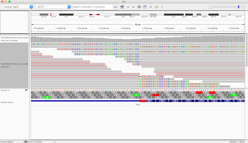
We verified manually that the viral sequence had been inserted correctly at the desired site, so that completed the synthetic data generation phase of the project. Time to move on to testing Pathseq on this data!
Finding the viral insertion with Pathseq
With the synthetic sample ready, we took it and ran it through the Pathseq pipeline to see whether it could find and correctly identify the HPV16 sequence. It did so easily – Pathseq created an output BAM (“final bam”) that contained all the high-quality non-host (i.e. HPV16) reads aligned to the microbe reference.
The next step was figuring out a way to identify these sites programmatically since Pathseq’s output was focused on microbial identification, while we were interested in the site of insertion with the host genome.
Identifying the insertion site
An obvious feature of an insertion site is that there are clusters of reads that are soft-clipped where the aligner is confident about part of the read but masks the other part of the alignment because it doesn’t match the reference. In IGV they appear as multicolored rainbow bands. The image above zoomed out looks like this:
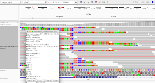
We discussed a few ways to identify these clusters: looking at CIGAR strings, SAM flags, and using a combination of utilities from other tools. We landed on using a combination of samtools and bedtools commands to filter down to only soft-clipped reads, grab the alignment chromosome and position, remove unaligned reads, and convert positions to padded intervals for easy viewing. You can see how we implemented this as part of the workflow we wrote for that part of the project; see the ClusterReads task. The output is a BED file that can be used in the following task for visualization.
Before moving on, I should note that we couldn’t just take the output BAM from Pathseq and go from there. We had to take the final BAM that contained all the non-host reads and align that back to the human genome so that the reads that were part human and part virus could be identified. We used BWASpark, which is a Spark-enabled implementation of BWA in GATK4. The pipeline ended up looking like this:
- FilterPathSeqBam
Remove reads to make it smaller- retain header and only soft-clipped reads that mapped to the virus taxon id - RevertSam
Remove mapping information and produce an unmapped BAM file (contents similar to a FASTQ file but in SAM format) - SortSam
Sort the data by queryname, i.e. the names of the sequence reads - BwaSpark
Align inserted reads back to the human reference - ClusterReads
Merge clustered loci together - IGV
Make snapshot images of the relevant regions
We settled on using IGV’s snapshot feature, inspired by a workflow authored by the Talkowski Lab for reviewing structural variants, to produce screenshots of putative insertion sites for manual review. We got some clues for how to do this by seeing how Steven Kelly and Michael Hall wrote their own IGV-snapshot-automator script. We knew exactly what software would be required thanks to their documentation. When we finally got the workflow to run, we hit another obstacle of getting the snapshot to show the right width and height in IGV. Through some thorough Googling, we found that providing an edited prefs.properties file was the solution.
To get this all working in Terra, we had to assemble a new Dockerfile that included prerequisite software for IGV, samtools, bedtools, and GATK. Here is what our file looked like:
FROM python:3
RUN apt-get update && apt-get install -y
bedtools
default-jre
xvfb
wget
samtools
&& rm -rf /var/lib/apt/lists/*
RUN wget https://data.broadinstitute.org/igv/projects/downloads/2.7/IGV_2.7.2.zip && unzip IGV_2.7.2.zip
CMD [“bash”]
ENV PATH /usr/local/bedtools/bin:$PATH
For a helpful primer on writing your own Dockerfile, see this recent article in PLOS Computational Biology (Nust et al., 2020).
Validation
After many hours of coding, troubleshooting, and tweaking, our pipeline was finally running end-to-end on our synthetic test sample. When the last workflow completed successfully, we were thrilled to find that it had correctly identified the insertion site and produced a single screenshot with a clean, colorful stack of the same soft-clipped reads we had observed in the original unfiltered synthetic BAM. While the site was notably lacking right-clipped reads, we decided to move forward rather than attempt to fine-tune the method to this artificial example, since this gave us the information we were looking for: the exact insertion site of the viral sequence.

We briefly reveled in this small victory, but we knew that our synthetic sample was unrealistic and we would need to validate the method using real sequencing data, which is bigger and messier. We scoured the literature for studies to benchmark against and happened upon a 2015 paper (Hu et al. 2015) that provided detailed tables of detected HPV insertions as well as their raw sequencing data.
Our initial attempts at running the full procedure on the data were met with mixed success. On the bright side, our pipeline did identify a number of sites reported in the study, as shown below.
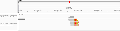
However, it both missed some real sites (false negatives) and generated spurious sites (false positives). We tweaked the filtering strategy and parameters to improve the results, a process that revealed some drawbacks of our method’s design, primarily stemming from its simplicity.
At the end of the day, it’s clear that our approach could be improved, for example by looking for read pairs where one read aligned to human and the other to virus. Nevertheless, for the intended scope of the project, we found that using simple soft-clipped read detection performed reasonably well and were quite happy with that result.
Assembling it all to make it usable by others – don’t forget the README!
Finally, we consolidated all of our work in a clean new workspace that we could share with the community in case it could be useful to someone working on similar problems. We created the documentation for the dashboard according to a Terra best practice template that we used internally. We set up the data model, imported the workflows and made them public, moved all the input files to a public Google bucket, and ran the workflows in the featured workspace to demonstrate each step. Anyone interested should be able to clone the workspace and run through all the steps based on the instructions in the dashboard, then build on this work from there.
You may wonder why we decided to move the files to a Google bucket separate from the workspace. This is to protect your work in case the workspace is ever accidentally deleted or updated – the output files will not be deleted and the file paths stay the same. We created a readme file in the public bucket so that users can understand how each of the files were generated and where they were used in the workspace. This was a good memory exercise, as I had forgotten how a few of these files were used.
Final thoughts
This project wasn’t a cake walk – there were a lot of bumps in the path. I had to leave out a lot of details about some of the issues we encountered to keep the story concise and readable, so the resulting narrative makes it sound a lot more straightforward than it was. Don’t be discouraged if it is your first time doing a project like this and you run into problems you don’t expect. It is a lot of work to make things work in the first place, then it takes some additional effort to make your research and methods easily understandable and reproducible. But it’s worth it, if only because your future self will thank you when questions come in and your brain forgets what you did 🙂
Please feel free to use or repurpose any of this code for your own work. I recommend cloning the workspace so you can try out the tools yourself and apply them to your own data with minimal effort, if that’s what’s you’re interested in doing.
If you’ve never used the Workflows feature in Terra, the Workflows Quickstart video on YouTube provides an end-to-end walkthrough of how to run a preconfigured workflow on example data in a workspace. You can also find complete documentation on this topic here.
Remember that if you run into any difficulties with Terra, my team is here specifically to help you get through it! For questions about this specific workspace, see the Contact information in the workspace dashboard.
Bibliography
Ewing, A., Houlahan, K., Hu, Y. et al. Combining tumor genome simulation with crowdsourcing to benchmark somatic single-nucleotide-variant detection. Nat Methods 12, 623–630 (2015). https://doi.org/10.1038/nmeth.3407
Hu Z, Zhu D, Wang W, et al. Genome-wide profiling of HPV integration in cervical cancer identifies clustered genomic hot spots and a potential microhomology-mediated integration mechanism. Nat Genet. 2015;47(2):158-163. https://doi.org/10.1038/ng.3178
Nüst D, Sochat V, Marwick B, Eglen SJ, Head T, Hirst T, et al. (2020) Ten simple rules for writing Dockerfiles for reproducible data science. PLoS Comput Biol 16(11): e1008316. https://doi.org/10.1371/journal.pcbi.1008316
Stephens ZD, Hudson ME, Mainzer LS, Taschuk M, Weber MR, Iyer RK (2016) Simulating Next-Generation Sequencing Datasets from Empirical Mutation and Sequencing Models. PLoS ONE 11(11): e0167047. https://doi.org/10.1371/journal.pone.0167047
Walker MA, Pedamallu CS, Ojesina AI, Bullman S, Sharpe T, Whelan CW, Meyerson M (2018) GATK PathSeq: a customizable computational tool for the discovery and identification of microbial sequences in libraries from eukaryotic hosts, Bioinformatics, Volume 34, Issue 24, 15 December 2018, Pages 4287–4289, https://doi.org/10.1093/bioinformatics/bty501