Samantha Zarate is a third-year PhD student in the computer science department at Johns Hopkins University in Baltimore, MD, working in the lab of Dr. Michael Schatz. As a member of the Telomere-to-Telomere consortium, she has been working for the last year to evaluate how the T2T-CHM13 reference genome affects variant calling with short-read data. In this guest blog post, Samantha explains what this entails, then walks us through the computational challenges she faced in implementing this analysis and how she solved them using Terra and the AnVIL.
Earlier this year, the Telomere-to-Telomere (T2T) consortium released the complete sequence of a human genome, unlocking the remaining 8% of the human genome reference unfinished in the current human reference genome and introducing nearly 200 million bp of novel sequence (Nurk, Koren, Rhie, Rautiainen, et al., 2021). For context, this is about as much novel sequence as in all of chromosome 3!
Within the T2T consortium, I led an analysis that demonstrated that the new T2T-CHM13 reference genome improves read mapping and variant calling for 3,202 globally diverse samples sequenced with short reads. We found that compared to the current standard, GRCh38, using this new reference mitigates or eliminates major sources of error that derived from incorrect assembly and certain idiosyncrasies of the samples previously used as the basis for reference construction. For example, the T2T-CHM13 reference includes corrections to collapsed segmental duplications, which are regions that previously appeared highly enriched for heterozygous paralog-specific variants in nearly all individuals due to the false pileup of reads from duplicated regions to a single location. This and other such corrections lead to a decrease in the number of variants erroneously called per sample when using the T2T-CHM13 reference genome. In addition, because we also added nearly 200Mbp of additional sequence, we discovered over 1 million additional high quality variants across the entire collection.
Our collaborators in the T2T consortium evaluated the scientific utility of our improved variant calling results. Excitingly, they found that the use of the new reference genome led to the discovery of novel signatures of selection in the newly assembled regions of the genome, as well as improved variant analysis throughout. This included reporting up to 12 times fewer false-positive variants in clinically relevant genes that have traditionally proved difficult to sequence and analyze.
Collectively, these results represent a significant improvement in variant calling using the T2T-CHM13 reference genome, which has broad implications for clinical genetics analyses, including inherited, de novo, and somatic mutations.
If you’d like to learn more about our findings and the supporting evidence, you can read the preprint on bioRxiv. In the rest of this blog post, I want to give some behind-the-scenes insight into what it took to accomplish this analysis — the computational challenges we faced, the decision to use Terra and the AnVIL, and how it went in practice — in case it might be useful for others tackling such a large-scale project for the first time.
Designing the pipeline and mapping out scaling challenges
To evaluate the T2T-CHM13 reference genome across multiple populations and a large number of openly accessible samples, we turned to the 1000 Genomes Project (1KGP), which recently expanded its scope to encompass 3,202 samples representing 602 trios and 26 populations around the world.
A team at the New York Genome Center (NYGC) had previously generated variant calls from that same dataset using GRCh38 as the reference genome (Byrska-Bishop et al., 2021), with a pipeline based on the functional equivalence pipeline standard established by the Centers for Common Disease Genomics (CCDG) and collaborators. The functional equivalence standard provides guidelines for implementing genome analysis pipelines in such a way that you can compare results obtained with different pipelines with confidence that any differences in the results are due to differences in specific inputs — such as a different reference genome — rather than to technical differences in the tools and methods employed.
By that same logic, if we followed their pipeline closely, we could perform an apples-to-apples comparison between their results and those we were going to generate with the T2T-CHM13 reference, and thus avoid having to redo the work that they had already done with GRCh38. As we implemented our pipeline, we only updated those elements that substantially improved efficiency without introducing divergences, and whenever possible, we used the same flags and options as the original study.
Pipeline overview
Conceptually, the pipeline consists of two main operations: (1) read alignment, in which we take the raw sequencing data for each sample and align, sort, and organize each read’s alignment to the reference genome, and (2) variant calling, in which we examine the aligned data to identify potential variants, first within each sample, then across the entire 1KGP collection. In practice, each of these operations consists of multiple steps of data processing and analysis, each with different computational requirements and constraints. Let’s take a closer look at how this plays out when you have to apply these steps to a large number of samples.
Read alignment
Read alignment involves aligning each read to the reference genome, plus a few additional steps to address data formatting and sorting requirements. When samples are sequenced using multiple flowcells, the data for each sample is subdivided into subsets called “read groups”, so we perform these initial steps for each read group. We then merge the aligned read group data per sample and apply a few additional steps: marking duplicate reads and compressing the alignment data into per-sample CRAM files. Finally, we generate quality control statistics that allow us to gauge the quality of the data we’re starting from.
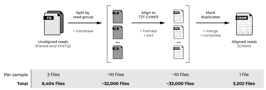
Our chosen cohort comprised genome sequencing data from 3,202 samples in the form of paired-end FASTQ files, meaning that our starting dataset consisted of 6,404 files. Applying the initial read alignment per read group would involve generating approximately 32,000 files at the “widest” point, to eventually produce 3,202 per-sample CRAM files, plus multiple quality control files for each sample. That’s a lot of files!
Variant calling
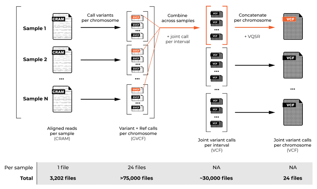
Read alignment is just the beginning. To generate variant calls across a large cohort, we have to decompose the process into two main operations, as described in the GATK Best Practices: first, we identify variants individually for each sample, then we combine the calls from all the samples in the cohort to generate overall variant calls in VCF format.
We performed the per-sample variant calling using a special mode of the GATK HaplotypeCaller tool that generates “genomic VCFs”, or GVCFs, which contain detailed information representing the entire genome (not just potentially variant sites, as you would find in normal VCF files). For efficiency reasons, we performed this step on a per-chromosome basis, generating over 75,000 files in total.
We then combined the variant calls from all the samples in the cohort for the “joint genotyping” analysis, which involves looking at the evidence at each possible variant site across all the samples in the cohort. This analysis produced the joint callset for the whole cohort, containing all the variant sites with detailed genotyping information and variant call statistics for each sample in the cohort.
The twist is that this step has to be run on intervals smaller than a whole chromosome, so now we’re combining per-chromosome GVCF files across all the samples, but producing per-interval joint-called VCFs — about 30,000 of them in total across the 24 chromosomes (more on that in a minute). Fortunately, we can then concatenate these files into just 24 per-chromosome VCF files.
And, finally, there’s a filtering step called variant recalibration (VQSR) that is done per-chromosome. This involves scoring variants to identify those with sufficiently high quality to use in downstream analysis, as opposed to those below this threshold, which we assume to be artifacts. The VCF files annotated with final variant scores and filtering information (PASS or otherwise) are the final outputs of the pipeline.
As you can imagine from this brief overview, joint genotyping alone presents various scaling challenges, and our T2T-CHM13 reference added an interesting complexity. Normally, for whole genomes, the GATK development team recommends defining the joint genotyping intervals by using regions with Ns in the reference as “naturally occurring” points where you don’t have to worry about variants spanning the interval boundaries. (For exomes, you can just use the capture intervals.)
However, the T2T-CHM13 reference doesn’t have any regions with Ns — that’s the whole point of a “telomere-to-telomere” reference! As a result, we developed a strategy that involves generating intervals of arbitrary length (100kb) and using 1kb padding intervals that we later trimmed off from the interval-level VCF files. The padding ensured that our variant calls didn’t suffer from edge effects, and we were able to verify that it didn’t make any difference to the final results.
Scaling up with Terra and the AnVIL
Implementing an end-to-end variant discovery analysis at the scale of thousands of whole genomes is not trivial, both in terms of basic logistics and computational requirements. We originally started out using the computing cluster available to us at Johns Hopkins University, but we realized very quickly that it would take too long and require too much storage for us to be successful on the timeline we needed to keep pace with the project. Based on our early testing, we estimated it would take many months, possibly up to a year, of computation to do all the data processing on our institutional servers.
So instead, we turned to AnVIL and the Terra platform, which promised massively scalable analysis, collaborative workspaces, and a host of other features to meet our needs.
Importing data
At the outset, we ran into some difficulties getting the starting dataset ready. We had originally planned to start from the NYGC’s version of the 1000 Genomes Project data (CRAM files aligned to GRCh38), which is already available through Terra as part of the AnVIL project. The idea was to revert those files to an unmapped state and then start our pipeline from there. However, we found that those files included some processing, such as replacing ambiguous nucleotides (N’s in the reads) with other bases, which we didn’t want — we wanted it to be as close to the raw data as possible to eliminate any possible biases introduced from GRCh38.
So we decided to shift gears and start from the original FASTQ files, which are available through the European Nucleotide Archive (ENA), and this is where we hit the biggest technical obstacle in the whole process. As I mentioned earlier, that dataset comprises 6,404 paired-end FASTQ files, which amount to about 100TB of compressed sequence data — for reference, that’s about 100,000 hours of streaming movies on Netflix in standard definition. Unfortunately, though not unexpectedly, the ENA didn’t plan on having people download that much data at once, so we had to come up with a way to transfer the data that wouldn’t crash their servers. We ended up using a WDL workflow to copy batches of about 100 files at a time to a Google bucket, managing the batches manually over several days. That was not fun.
Executing workflows at scale and collaborating
After that somewhat rocky start, however, running the analysis itself was surprisingly smooth. We implemented the pipeline described above as a set of WDL workflows, and we used Terra’s built-in workflow execution system, called Cromwell, to run them on the cloud.
Scaling up went well, especially considering the alternative to using Terra was using our university’s HPC, which is subject to limited quotas, traffic restrictions from other users and equipment failures in a way that Google Cloud servers aren’t. The push-button capabilities of Terra let us scale up easily and rapidly: after verifying the success of our WDLs on a few samples, we could move on to processing hundreds or thousands of workflows at a time. It took us about a week to process everything, and that was with Google’s default compute quotas in place (eg max 25,000 cores at a time), which can be raised on request.
We also really appreciated how easy it was to collaborate with others. Working in a cloud environment, it was very easy to keep our collaborators informed on progress and share results with members of the consortium. If we had been using our institutional HPC, which does not allow access to external users, we would have had to copy files to multiple institutions to provide the same level of access.
More generally, we found that the reproducibility and reusability of our analyses have increased significantly. Having implemented our workflows in WDL to run in Terra, we can now publish them on GitHub, knowing that anyone can download them and replicate our analysis on their infrastructure, as Cromwell supports all major HPC schedulers and public clouds. We have also published the accompanying Docker image, so the environment in which we are running our code is also reproducible. With all of the materials we used for this analysis available publicly in Terra and relevant repositories, any interested party has all of the tools they need to fully reproduce our analysis and extend it for their purposes.
Room for improvement
One of the things we didn’t like so much was having to select inputs and launch workflows manually in the graphical web interface. That was convenient for initial testing, but we would have preferred to use a CLI environment to launch and manage workflows once we moved to full-scale execution. We only learned after completing the work that Terra has an open API and that there is a Python-based client called FISS that makes it possible to perform all the same actions through scripted commands. The FISS client is covered in the Terra documentation (there’s even a public workspace with a couple of tutorial notebooks) but we never saw any references to it until it was pointed out to us by someone from the Terra team, so this feature needs more visibility.
We’d also love to see more functionality added around data provenance. The job history dashboard gives you a lot of details if you’re looking at workflow execution records. However, you can’t select a piece of data and see how it was generated, by what version of the pipeline, and so on. Being able to identify the source of a given file, notably the workflow that created it as well as the parameters used, would be greatly helpful for tracing back files, especially when a workflow has been updated and files need to be re-analyzed. Or as another example, when two or more files are named XXX.bam, it’s very helpful to be able to tell which one is the final version in a way other than writing down the time each respective workflow was launched.
Finally, as mentioned above, transferring the data from ENA was painful, so we’d love to see some built-in file transfer utilities to make that process more efficient. There is currently no built-in way to obtain data from a URL or FTP link; implementing a universal file fetcher would help users move data into Terra more efficiently.
Conclusions
Scientifically, our analysis strongly supports the use of T2T-CHM13 for variant calling. We find impressive improvements in both alignment and variant calling, as CHM13 both resolves errors in GRCh38 and adds novel sequences. Our collaborators within the T2T consortium performed further analysis using the joint genotyped chromosome-wide VCF files and also found improvements in medically relevant genes and the overall accuracy of variant calling genomewide, thus demonstrating the utility of T2T-CHM13 in clinical analysis.
From a technical standpoint, this was our first time using Terra for large-scale analysis, and we found that the benefits of Terra outweighed the few pain points. Compared to a high-performance cluster, Terra is much more user-friendly for scaling up, reproducing workflows, and collaborating with others across institutions. We have noted some quality-of-life changes that would improve Terra’s useability, and we are confident that if these are implemented, Terra would become an even stronger option in the cloud genomics space.
Moving forward, we have been buoyed by the quality of the T2T-CHM13 reference, and we plan on using it for future large-scale analyses using Terra. As we demonstrate here, CHM13 is easy to use as a reference for large-scale genomic analysis, and we hope that both the clinical and research genomics communities use it to improve their own workflows.
References
Byrska-Bishop, M. et al. (2021) ‘High coverage whole genome sequencing of the expanded 1000 Genomes Project cohort including 602 trios’, bioRxiv. doi: 10.1101/2021.02.06.430068.
Nurk, S. et al. (2021) ‘The complete sequence of a human genome’, bioRxiv. doi: 10.1101/2021.05.26.445798.